FPGA Design
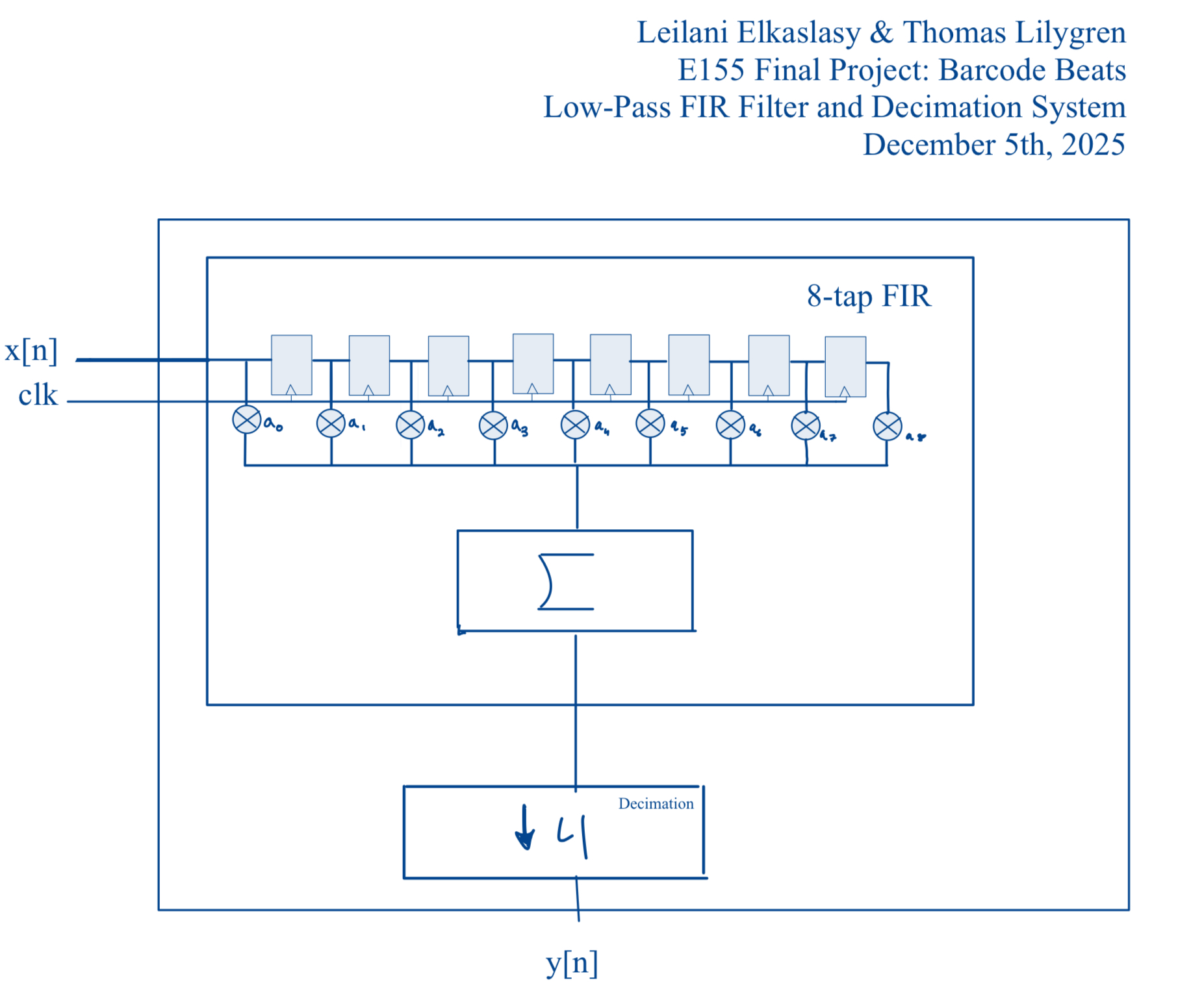
The FPGA conducts digital signal processing on the input serial square wave generated by the NetumScan 1D Barcode Scanner’s infrared receiver. Since the The FPGA conducts and eight-tap Finite Impulse Response (FIR) low-pass filter with a decimation factor of four. The FIR filter employs carefully optimized tap coefficients and convolution to smooth out high-frequency jitters and stark frequency shifts by implementing a weighted frequency average. The governing equation for FIR filtering is outlined with the equation below.
\[ y[n] = \sum_{k=0}^{M-1} h[k]\,x[n-k] \]
Filter Design with Shift Register and Decimation
The FPGA implements convolution via a shift register with eight flip-flops. Only eight registers can be accomodated since this is the maximum number of multipliers within the FPGA’s DSP block. A 24 MHz clock frequency is initiated with the device’s internal high-speed oscillator (HSOSC) and a counter is used to divide this frequency to a 48 kHz sampling frequency. Upon each rising edge of the of the sampling signal, a new sample of the input wave is taken an propagates through the shift register. At each stage in the shifting process, signals output from each flip-flop are multiplied by designated signed tap coefficients and summed to produce a tuning word. The factor of 4 decimation reduces the sampling rate to 12 kHz, so the tuning word is only updated every four samples. The downsampling provides added fidelity for future SPI communication, controls the speed for which the frequency modulation on the MCU occurs, and enhances overall signal quality.
After two decimation cycles, the shift register fills with new barcode data and produces a new 32-bit tuning word that is sent to the MCU over 4 8-bit SPI transactions to govern direct digital synthesis (DDS). More information regarding the process can be found in the MCU design description.
Tap Coefficients
The tap coefficients were generated using a MATLAB script that swept through potential coefficient options to find the “roundest” combination of coefficients, indicating greater attenuation of higher harmonic frequencies. Refer to Table 1 below that outlines the optimal coefficient weights.
Table 1: Tap Coefficient Weights
| Coefficient | Weight |
|---|---|
| a0 | 10 |
| a1 | 33 |
| a2 | 85 |
| a3 | 127 |
| a4 | 127 |
| a5 | 85 |
| a6 | 33 |
| a7 | 10 |
Filter Performance Simulations in MATLAB
FIR filter coefficient calculation and visualization
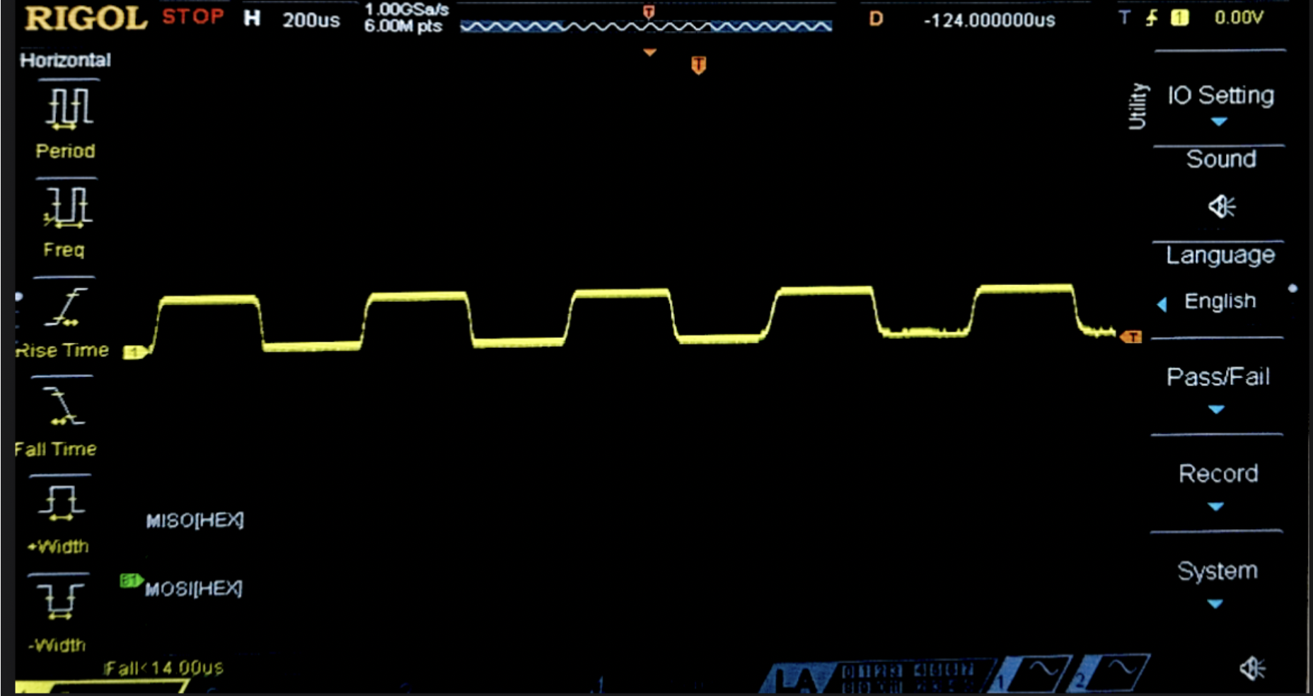
To determine the optimal 8-tap FIR low-pass filter coefficients for smoothing, the raw signal from a uniform barcode pattern was measured on the oscilloscope (Figure 3). The signal demonstrated an approximate 1.2 kHz square wave frequency around which the MATLAB script was optimized. While the signal frequency depends on the speed and height of the scanner as well as the pattern it reads, this value was deemed as a sufficient baseline for modeling purposes.
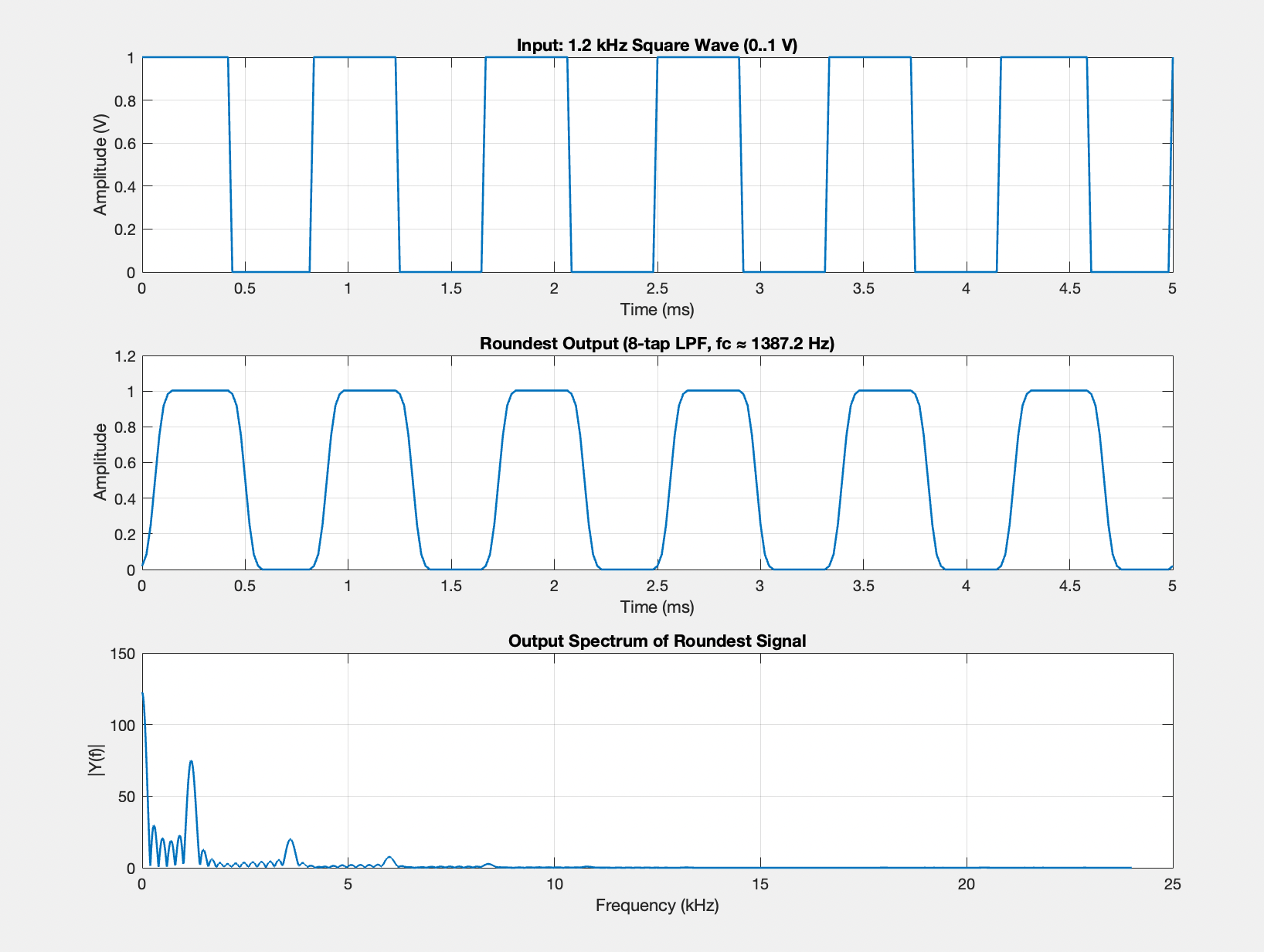
This script sweeps through a range of potential cut-off frequencies and designs the subsequent 8-tap filter using fir1 (a built-in MATLAB function that designs FIR filters through the window method). The script then converts the coefficients to signed 8-bit integers that are compatible with the FPGA hardware. These coefficients were applied to a simulated 1.2 kHz square wave input and the Total Harmonic Distortion (THD) of the filtered wave form is measured through the amplitude of the fundamental frequency and its odd harmonics. The applied cutoff frequency that produces the lowest THD value is represented by the smoothest possible output given 8 coefficients. Visualization of the optimal tap weights and the corresponding filtering they introduce is demonstrated in Figure 4.
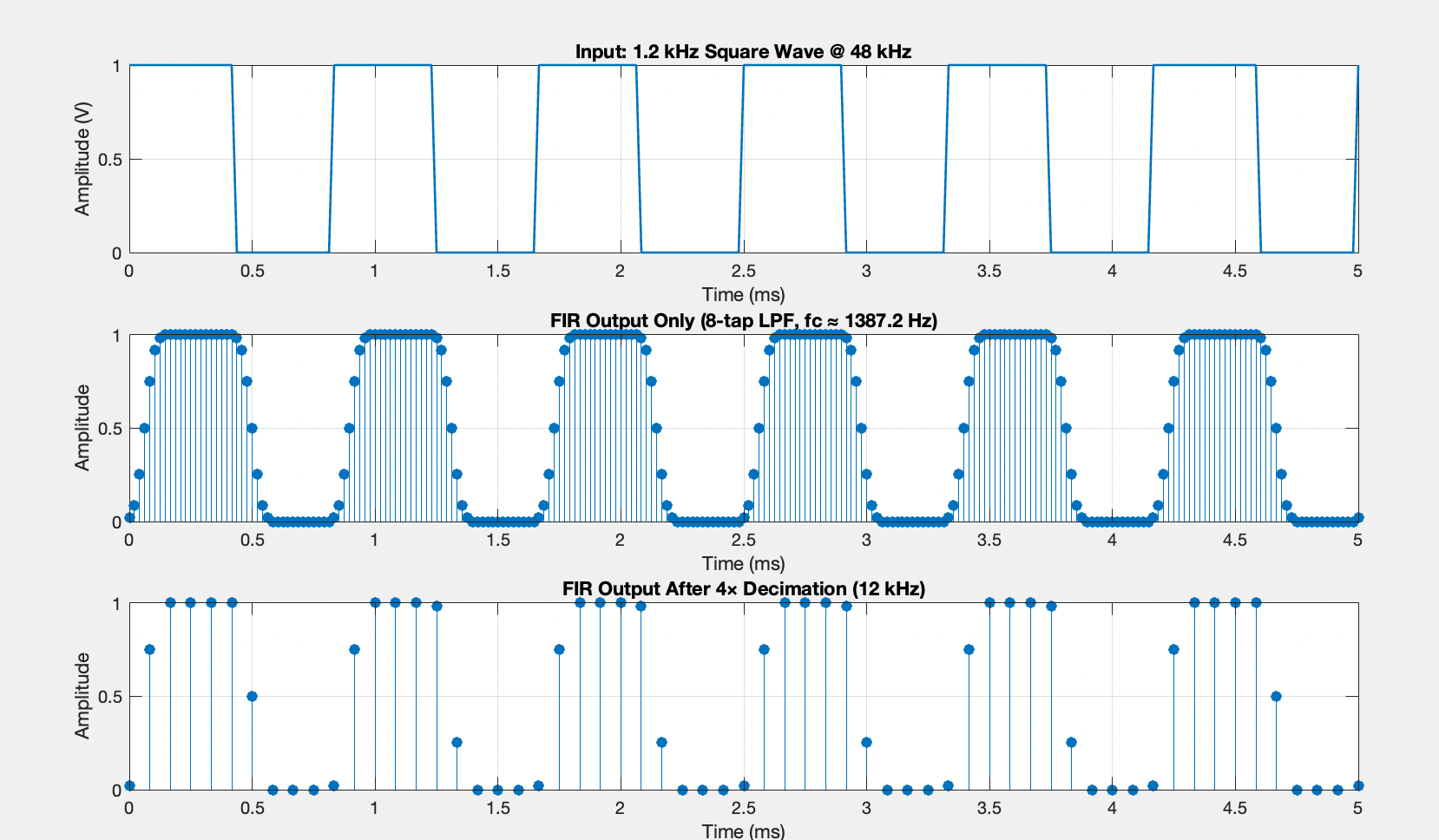
Decimation Visualization
The impacts from the 4x decimated sampling frequency were also visualized using the MATLAB script (Figure 4). The first plot shows and example 1 kHz input square wave that the barcode scanner would receive, the second shows the same square wave sampled at the original 48 kHz frequency, and the third plot shows the downsampled 12 kHz wave.